Mean-Reversion Volatility Filters Part Two: Since 2011

On my previous post, Mean-Reversion Volatility Filters, I used a dynamic volatility filter to filter out trades within  a short-term mean reversion system. I came to the conclusion that low vol was conducive for short term mean reversion performance. However, it’s commonly discussed how the market has shifted dynamics some time after the 2007-2008 financial crisis. In this post I revisit the tests ran in my previous post, testing from 1/1/2011 – 4/28/2013 rather than 1/1/1995 – 4/28/2013. The charts displayed below are 10-trade moving average of % profit from 1/1/1995-4/28/2013.

Results

IBS

Rules (Base-Case):

• Buy if 3-Day IBS < 40
• Sell if 3-Day IBS > 40
• Avg. Trade: 0.53%

Rules (High Vol):

• Buy if 3-Day IBS < 40 AND HV(5) > HV(20)
• Sell if 3-Day IBS > 40
• Avg. Trade: 0.68%

Rules (Low Vol):

• Buy if 3-Day IBS < 40 and HV(5) < HV(20)
• Sell if 3-Day IBS > 40
• Avg. Trade: 0.38%

RSI

Rules (Base-Case):

• Buy if 2-Day RSI< 50
• Sell if 2-Day RSI > 50
• Avg. Trade: 0.21%

Rules(High Vol):

• Buy if  2-Day RSI< 50 and HV(5) > HV(20)
• Sell if 2-Day RSI > 50
• Avg. Trade: 0.40%

Rules(Low Vol):

• Buy if  2-Day RSI< 50 and HV(5) < HV(20)
• Sell if 2-Day RSI > 50
• Avg. Trade: 0.10%

Conclusion

Without looking at the charts, it may seem like post 2011, this volatility filter, like many strategies, has completely changed. However after looking at the charts of a rolling 10-trade moving average of % profit. the results become more inconclusive. It seems much more likely that the short term test results are due to unrepresentative and small sample size, rather than a change in volatility filter performance.

 

Mean-Reversion Volatility Filters

Due to the result’s of this MarketSci post, which imply that short-term mean reversion performs better during low volatility versus high volatility, I decided to revisit volatility filters. In Mean-Reversion within Regimes, I previously concluded that high volatility, not low volatility was more conducive to mean-reversion strategies. To test for low volatility/high volatility I decided to use a different filter. Last time I used a static test (60-Day Historical Volatility > 0.01 = High Volatility, <0.01 = Low Volatility). This time I will use a more dynamic filter, which compares short-term volatility to mid-term volatility.

Results

• Testing on SPY from 1/1/1995- 4/28/2013

IBS

Rules (Base-Case):

• Buy if 3-Day IBS < 40
• Sell if 3-Day IBS > 40
• Avg. Trade: 0.56%

Rules (High Vol):

• Buy if 3-Day IBS < 40 AND HV(5) > HV(20) 
• Sell if 3-Day IBS > 40
• Avg. Trade: 0.39%

Rules (Low Vol):

• Buy if 3-Day IBS < 40 and HV(5) < HV(20)
• Sell if 3-Day IBS > 40
• Avg. Trade: 0.68%

RSI

Rules (Base-Case):

• Buy if 2-Day RSI< 50
• Sell if 2-Day RSI > 50
• Avg. Trade: 0.32%

Rules(High Vol):

• Buy if  2-Day RSI< 50 and HV(5) < HV(20)
• Sell if 2-Day RSI > 50
• Avg. Trade: 0.27%

Rules(Low Vol);

• Buy if  2-Day RSI< 50 and HV(5) < HV(20)
• Sell if 2-Day RSI > 50
• Avg. Trade: 0.37%

Conclusion

It seems from this, in combination with my previous conclusion from Mean-Reversion within Regimes, that the specific filter used for volatility has a large influence on profitability. One thing I realized is that there may be different exposures for low vol vs high vol (meaning that a high volatility filter may allow for more trades, resulting in a higher CAGR) which could result in the discrepancy in results (that is why I used Avg. Trade rather than CAGR this time), but even after re-running the different tests under the same conditions, high vol had a higher Avg. Trade vs low vol.

Short Term Trend-Following within Mean-Reversion Trading

A while ago CSS Analytics had a post titled Improving Trend-Following Strategies with Counter-Trend Entries, which discusses using a mean-reversion indicator to filter out trades from a trend-following system. It got me thinking about using trend-following philosophy with mean-reversion trading systems. Mean-reversion is based off of buying dips; however, many times oscillators and other mean-reversion indicators are too quick when calling a market dip, and end up losing money the next day or so of an entered trade. To counter-act this tendency, why not use the old trend-following adage to only buy if the trend is up?

To test this, I used my favorite mean-reversion system:

• Buy if DV2 < 50
• Sell if DV2 > 50
• No Shorting

with two variations. Before I go into the two variations, I will post the results of this simple mean-reversion system traded on SPY from 1/1/2000 – 1/1/2013 for comparison. All results are  frictionless:

Variation One

• Buy if DV2 < 50 AND Today’s DV2 is ABOVE Yesterday’s DV2
• Sell if DV2 > 50
• No Shorting

Variation Two

• Buy if DV2 < 50 AND Today’s Close is ABOVE Yesterday’s Close
• Sell if DV2  > 50
• No Shorting

Variation One is vastly superior to the simple DV2 strategy when one factors for exposure and maximum drawdown. Variation Two has slightly lower returns when adjusted for exposure, but the maximum drawdown is reduced by 1/3. Using trend-following techniques to filter out bad trades can vastly increase risk-adjusted returns in mean-reversion trading systems.

Mean Reversion Trading in Moderation

Simple mean-reversion trading strategies in US equities have performed poorly since 2010/2011. Mean reversion is not dead, it never will be, but it may expressed differently than previously. Mean reversion prior to 2010, existed mainly in the form of extremes. The more extreme a pullback, the higher chance for a huge reversal. To test this, I ran 10 different frictionless  tests on SPY (from Yahoo! Finance) from 1/1/2000 – 1/1/2010.

Rules:

• Buy if the 250-day DV2 is greater than a threshold AND if it is less than the threshold + 10 (this means I will only buy if the DV2 is within a certain 10 point range).
• Sell the next day.
•  It is worth noting here that I have an option on in AmiBroker that prevents me from entering buy orders the same day that I enter sell orders, which will lower the overall exposure of these systems.

Here are the results:

We can clearly see that the returns are largely derived from the 1-11 bucket, meaning that extreme mean reversion was the source of returns. In the past 3 years, mean reversion exists in more moderate forms. Extreme pullbacks no longer indicate large reversals, but moderate pullbacks are more indicative of future gains. To test this, I ran the same test from 1/1/2010 – 1/1/2013:

The returns for the past three years are from the 31-41, 41-51, and 51-61 bucket. The 1-11 bucket went from a 6% CAGR to a -2% CAGR.

Here are the rules for another test I ran. This should be the result of the above rules if I allowed entries to be entered the same day as exits.

Rules:

• Buy if the 250-day DV2 is greater than a threshold AND if it is less than the threshold + 10 (this means I will only buy if the DV2 is within a certain 10 point range).
• Sell if the 250-day DV2 is less than a threshold OR if it is more than the threshold + 10

Results for 1/1/2000 – 1/1/2010:

Results for the same test for 1/1/2010 – 1/1/2013:

This is only a preliminary test over SPY, but it does lead to avenues for further research.

Scaling In (Part Three): IBS & RSI

On my previous two posts regarding pyramiding (first post, second post), I tested three different entry methodologies using a DV2 across multiple securities. To obtain further results of the entry methodology within mean-reversion trading systems, I will test it on a simple IBS system and 2-day RSI system.

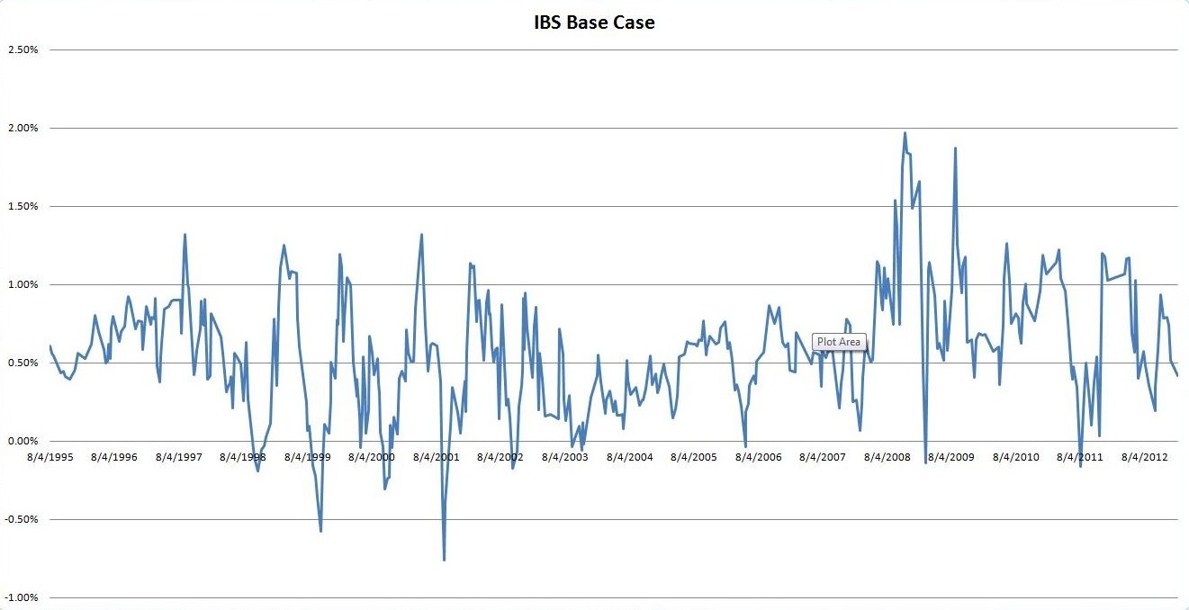
IBS

SPY

Default (Buy 100% of equity when IBS < 45, Sell 100% of position when IBS > 50):

• Exposure: 42.51%
• CAGR: 10.33%
• MDD: 25.28%

Purchase at first Dip (Buy 100% of equity the first day the close is less than the close of the day IBS < 45, Sell 100% of position when IBS > 50):

• Exposure: 16.57%
• CAGR: 7.38%
• MDD: 15.63%

Scale In(Buy 50% of equity when IBS < 45, Buy 50% of equity more the first day the close is less than the close of the day IBS < 45, Sell 100% of position when IBS > 50):

• Exposure: 28.59%
• CAGR: 8.77%
• MDD: 19.49%

Nasdaq-100

Default(Buy 6% of equity when IBS < 45, Sell 100% of position when IBS > 50):

• Exposure: 77.56%
• CAGR: 24.06%
• MDD: 41.65%

Purchase at a Dip(Buy 18% of equity the first day the close is less than the close of the day IBS < 45, Sell 100% of position when IBS > 50):

• Exposure: 68.46%
• CAGR: 41.04% (Better than DV2)
• MDD: 32.76%

Scale In(Buy 3% of equity when IBS < 45, Buy 3% of equity more on each subsequent day the close is less than the close of the first day IBS < 45, Sell 100% of position when IBS > 50):

• Exposure: 71.42%
• CAGR: 29.46%
• MDD: 40.33%

Individual Nasdaq-100

Lastly, I tested a system individually on each Nasdaq-100 stock.

Default(Buy 100% of equity when IBS < 45, Sell 100% of position when IBS > 50):

• Average of Exposure: 44.96%
• Standard Deviation of Exposure: 2.87%
• Average of CAGR: 14.58%
• Standard Deviation of CAGR: 16.04%
• Average of MDD: 29.14%
• Standard Deviation of MDD: 16.11%

Purchase at first Dip(Buy 100% of equity the first day the close is less than the close of the day IBS < 45, Sell 100% of position when IBS > 50):

• Average of Exposure: 17.04%
• Standard Deviation of Exposure: 2.55%
• Average of CAGR: 3.94%
• Standard Deviation of CAGR: 9.06%
• Average of MDD: 21.57%
• Standard Deviation of MDD: 14.23%

Scale In(Buy 50% of equity when IBS < 45, Buy 50% of equity more the first day the close is less than the close of the first day IBS < 45, Sell 100% when IBS > 50):

• Average of Exposure: 30.82%
• Standard Deviation of Exposure: 3.77%
• Average of CAGR: 9.38%
• Standard Deviation of CAGR: 11.37%
• Average of MDD: 23.76%6.96/25.2
• Standard Deviation of MDD: 14.97%

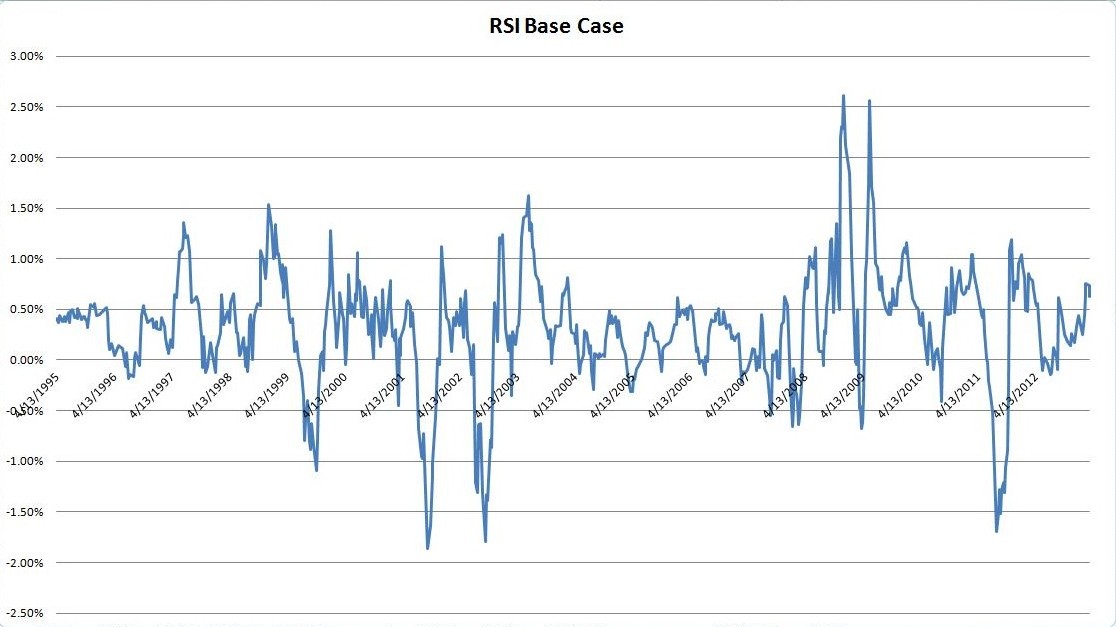
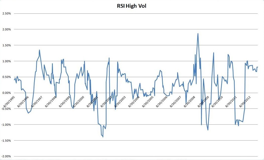
RSI

SPY

Default(Buy 100% of equity when RSI < 50, Sell 100% of position when RSI > 50):

• Exposure: 44.40%
• CAGR: 9.20%
• MDD: 25.90%

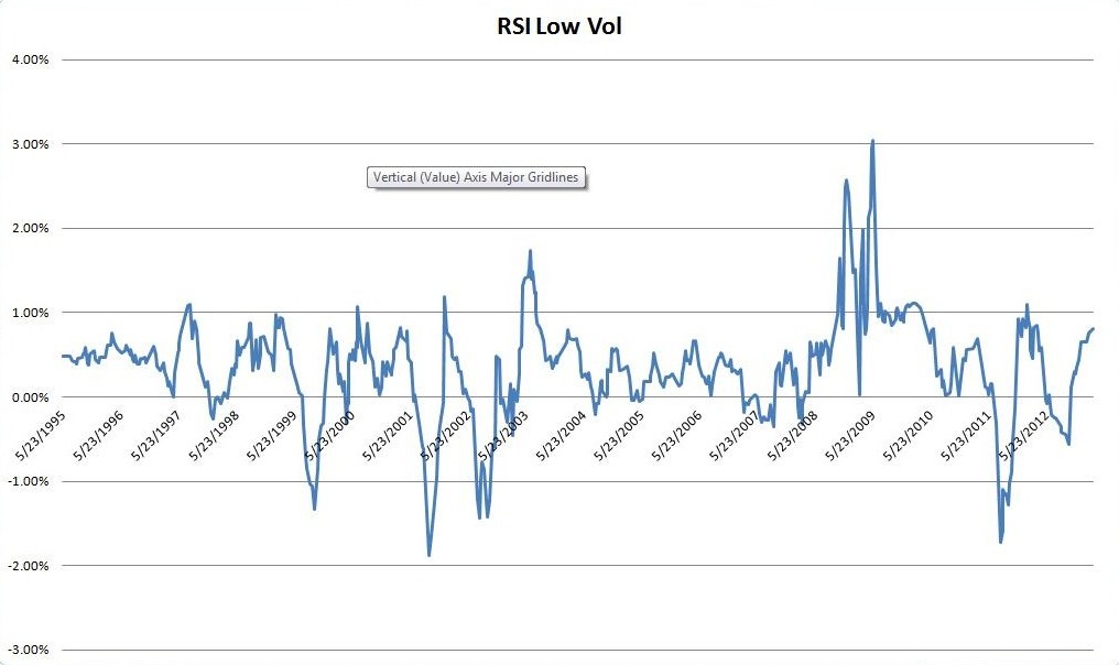
Purchase at first Dip(Buy 100% of equity the first day the close is less than the close of the day RSI < 50, Sell 100% of position when RSI > 50):

• Exposure: 25.27%
• CAGR: 6.96%
• MDD: 19.80%

Scale In(Buy 50% of equity when RSI < 50, Buy 50% of equity more the first day the close is less than the close of the day RSI < 50, Sell 100% of position when RSI > 50):

• Exposure: 34.87%
• CAGR: 8.19%
• MDD: 20.34%

Nasdaq-100

Default(Buy 2% of equity when RSI < 50, Sell 100% of position when RSI > 50):

• Exposure: 68.08%
• CAGR: 19.74%
• MDD: 41.65%

Purchase at a Dip(Buy 6% of equity the first day the close is less than the close of the day RSI < 50, Sell 100% of position when RSI > 50):

• Exposure: 71.59%
• CAGR: 32.28%
• MDD: 31.40%

Scale In(Buy 3% of equity when RSI < 50, Buy 3% of equity more on each subsequent day the close is less than the close of the first day RSI < 50, Sell 100% of position when RSI > 50):

• Exposure: 69.75%
• CAGR: 29.68%
• MDD: 34.54%

Individual Nasdaq-100

Default(Buy 100% of equity when RSI < 50, Sell 100% of position when RSI > 50):

• Average of Exposure: 44.73%
• Standard Deviation of Exposure: 5.85%
• Average of CAGR: 9.03%
• Standard Deviation of CAGR: 11.96%
• Average of MDD: 60.83%
• Standard Deviation of MDD: 21.23%

Purchase at first Dip(Buy 100% of equity the first day the close is less than the close of the day RSI < 50, Sell 100% of position when RSI > 50):

• Average of Exposure: 26.98%
• Standard Deviation of Exposure: 3.39%
• Average of CAGR: 9.03%
• Standard Deviation of CAGR: 10.24%
• Average of MDD: 50.77%
• Standard Deviation of MDD: 20.91%

Scale In(Buy 45% of equity when RSI < 50, Buy 45% of equity more the first day the close is less than the close of the first day RSI < 50, Sell 100% when RSI > 50):

• Average of Exposure: 37.99%
• Standard Deviation of Exposure: 2.19%
• Average of CAGR: 10.27%
• Standard Deviation of CAGR: 11.25%
• Average of MDD: 55.67%
• Standard Deviation of MDD: 21.57%

Conclusion

At a quick glance, it’s clear that purchasing at the first dip for mean reversion trading systems seems to offer the best risk/reward ratio. At times, the differences are marginal, but after factoring for exposure, purchasing at first dip exceeds scaling in in (5/6) tests and the default trading system in (5/6) tests, on an absolute and risk-adjusted basis.

Scaling In (Part Two)

On Scaling In: Confusion (Part One) regarding pyramiding, I discussed the possibility of the Avg. Profit/Loss% performance metric being a subpar measure of system performance. To get a better understanding of system performance of buying on pullbacks, scaling, and default mean reversion trading systems, I decided to use two other performance metrics (three if you consider exposure a performance metric).

SPY

Default(Buy 100% of equity when DV2 < 50, Sell 100% of position when DV2 > 50):

• Exposure: 49.61%
• CAGR: 13.03%
• MDD: 27.82%

Purchase at first Dip(Buy 100% of equity the first day the close is less than the close of the day DV2 < 50, Sell 100% of position when DV2 > 50):

• Exposure: 25.52%
• CAGR: 9.36%
• MDD: 19.80%

Scale In(Buy 50% of equity when DV2 < 50, Buy 50% of equity more the first day the close is less than the close of the day DV2 < 50, Sell 100% of position when DV2 > 50):

• Exposure: 37.64%
• CAGR: 11.50%
• MDD: 21.94%

Nasdaq-100

Default(Buy 2% of equity when DV2 < 50, Sell 100% of position when DV2 > 50):

• Exposure: 69.75%
• CAGR: 33.44%
• MDD: 27.70%

Purchase at a Dip(Buy 6% of equity the first day the close is less than the close of the day DV2 < 50, Sell 100% of position when DV2 > 50):

• Exposure: 68.07%
• CAGR: 37.03%
• MDD: 29.98%

Scale In(Buy 1% of equity when DV2 < 50, Buy 1% of equity more on each subsequent day the close is less than the close of the first day DV2 < 50, Sell 100% of position when DV2 > 50):

• Exposure: 68.43%
• CAGR: 38.03%
• MDD: 27.22%

Individual Nasdaq-100

Default(Buy 100% of equity when DV2 < 50, Sell 100% of position when DV2 > 50):

• Average of Exposure: 44.58%
• Standard Deviation of Exposure: 6.43%
• Average of CAGR: 15.76%
• Standard Deviation of CAGR: 10.68%
• Average of MDD: 54.95%
• Standard Deviation of MDD: 19.95%

Purchase at first Dip(Buy 100% of equity the first day the close is less than the close of the day DV2 < 50, Sell 100% of position when DV2 > 50):

• Average of Exposure: 24.22%
• Standard Deviation of Exposure: 2.69%
• Average of CAGR: 9.81%
• Standard Deviation of CAGR: 8.22%
• Average of MDD: 46.23
• Standard Deviation of MDD: 18.34

Scale In(Buy 50% of equity when DV2 < 50, Buy 50% of equity more the first day the close is less than the close of the first day DV2 < 50, Sell 100% when DV2 > 50):

• Average of Exposure: 36.82%
• Standard Deviation of Exposure: 2.18%
• Average of CAGR: 14.42%
• Standard Deviation of CAGR: 9.66%
• Average of MDD: 49.77%
• Standard Deviation of MDD: 19.06%

Conclusion

The differences between each method seems negligible. Personally, I plan to use the purchase at first dip method. Even though the scaling in method and the first dip method have similar CAGRs after factoring for exposure (the first dip method has marginally higher CAGRs for 2/3 tests), the scaling in method will have higher commissions and slippage costs. The first dip method also had a lower MDD on 2/3 of the tests, but that has little to do with my decision. In Scaling In (Part Three) I reach similar conclusions, testing these entry methodologies across two other simple mean-reversion trading systems.

Scaling In: Confusion (Part One)

I’ve never quite understood the rational for scaling in for mean-reversion type trading systems. Scaling in for trend-following trades is simple and intuitive. By trading only a portion of your allocated capital at first, you can wait for further confirmation of the trend until you trade the rest of your capital. The trade off is that you will receive a worse entry price. However, for mean-reversion trading strategies you receive a better entry price at the cost of less trading opportunities. This may seem obvious, but my question is why scale in at all? Why not just place 100% of the order on the first or the second scaled-in purchase signal? Intuitively, it seems like either purchasing 100% of the position at the initial buy signal, or purchasing 100% of the position at the first dip after the buy signal, would produce the best results, and scaling in would only produce a return somewhere in between the other two results.  To test this out, I backtested three frictionless versions of a simple long-only DV2 system on SPY from 1/1/2000 – 2/5/2013.

Default(Buy 100% of equity when DV2 < 50, Sell 100% of position when DV2 > 50):

• Number of trades: 573
• Avg. Profit/Loss %: 0.30%

Purchase at first Dip(Buy 100% of equity the first day the close is less than the close of the day DV2 < 50, Sell 100% of position when DV2 > 50):

• Number of trades: 292
• Avg. Profit/Loss %: 0.43%

Scale In(Buy 50% of equity when DV2 < 50, Buy 50% of equity more the first day the close is less than the close of the day DV2 < 50, Sell 100% of position when DV2 > 50):

• Number of trades: 575
• Avg. Profit/Loss%: 0.55%

I tested a similar system on all Nasdaq-100 stocks (that are currently listed as of 2/15/2013. Does contain survivorship bias).

Default(Buy 2% of equity when DV2 < 50, Sell 100% of position when DV2 > 50):

• Number of trades: 38998
• Avg. Profit/Loss%: 0.52%

Purchase at a Dip(Buy 6% of equity the first day the close is less than the close of the day DV2 < 50, Sell 100% of position when DV2 > 50):

• Number of trades: 13056
• Avg. Profit/Loss%: 0.59%

Scale In(Buy 1% of equity when DV2 < 50, Buy 1% of equity more on each subsequent day the close is less than the close of the first day DV2 < 50, Sell 100% of position when DV2 > 50):

• Number of trades: 37342
• Avg. Profit/Loss%: 1.48%

Lastly, I tested a system individually on each Nasdaq-100 stock.

Default(Buy 100% of equity when DV2 < 50, Sell 100% of position when DV2 > 50):

• Average of Avg. Profit/Loss%: 0.50%
• Standard Deviation of Avg. Profit/Loss%: 0.22%

Purchase at first Dip(Buy 100% of equity the first day the close is less than the close of the day DV2 < 50, Sell 100% of position when DV2 > 50):

• Average of Avg. Profit/Loss%: 0.57%
• Standard Deviation of Avg. Profit/Loss%: 0.34%

Scale In(Buy 50% of equity when DV2 < 50, Buy 50% of equity more the first day the close is less than the close of the first day DV2 < 50, Sell 100% when DV2 > 50):

• Average of Avg. Profit/Loss%: 1.07%
• Standard Deviation of Avg. Profit/Loss%: 0.26%

The results produce a unanimous conclusion across all three tests: scaling in produces the best average profit/loss. The only possible explanation I can think of is this: Avg. Profit/Loss % is independent of position sizing (meaning that a 2% gain on 50% of equity is the same as a 2% gain on 100% of equity) so scaling in would produce an outsized Avg. Profit/Loss% because the system contains the trades that never face a loss throughout its life, while being able to average down on trades that do contain a loss. Since these two types of trades will be weighted equally in the calculation of Avg. Profit/Loss% (because of the fact that the metric is independent of position sizing) it substantially boosts Avg. Profit/Loss%. In essence, I picked a subpar performance metric (Scaling In (Part Two) is a posts that run the same tests with a different performance metric). If anyone has any other insights as to why this occurs, please comment below!

RSI of Volatility Indicator

It’s common knowledge by now that low volatility is conducive to bullish behavior and high volatility is conducive to bearish behavior. To create a trading system that would short bursts of high volatility and buy short periods of low volatility I took the 5-day RSI of the daily Close-Open Range.

Edit: Commenter Ramiro called to my attention that I do not actually take the RSI of the Close-Open range, just the Close-Open. I’m actually measuring the magnitude AND the direction, meaning that this is just simply another mean-reversion indicator, NOT a volatility indicator.

To turn my indicator into a trading system, I optimized buy and sell threshold (1-100) on SPY from 1/1/2000 – 12/29/2012. I optimized a long-only version of the system. Here is a picture of the 3D optimization with CAGR on the z-axis.

Buy Threshold

Sell Threshold

There is a small hilly region near the middle. I chose 40 as my buy threshold and 55 as my sell threshold since they are round numbers within the hilly region.

One thing peculiar that I noticed, but can’t seem to explain is that there are two of every set of system statistics, and the only difference is 1) the parameters of buy/sell threshold are switched and 2) the number of trades:

After some pondering I noticed that it might be because some of the buying is negligible. For example, if we have a 40/60 threshold then we will buy if the RSI is at 30, regardless if the 40 or the 60 is the buy threshold. However, the problem that I came across is that if the RSI is at 30 today, but is at 50 tomorrow, then we will buy & hold for a 40/60 threshold (buy when RSI < 40 and sell when RSI > 60), but we will buy & sell for a 60/40 threshold ( buy when RSI < 60 and sell when RSI > 40). I can’t seem to figure out why there each set of system statistics has a twin.

Next, I optimized the short and cover threshold (1-100) on the same data, using a short-only version of the system. Here is a picture of the 3D optimization with CAGR on the z-axis.

Short Threshold

Cover Threshold

There is another small hilly region near the middle. I chose 55 as my short threshold and 40 as my cover threshold since they are round numbers within the hilly region.

The peculiarity of the long only side of the system does not seem to exist on the short side.

Here is the optimized equity curve with a system of the following rules:

• Buy RSI < 40
• Sell RSI > 55
• Cover RSI < 40
• Short RSI > 55

The equity curve looks similar to that of many mean-reversion trading systems.

To check for robustness, I tested this system on multiple ETFs from 1/1/2000 – 12/29/2012.

For further robustness, I tested this system using different lengths of RSI on SPY.

One of my concerns is the success of the system since 2010, since many systems seemed to have performed differently or even completely stopped working from around that period. Here is the performance of the system on multiple markets from 1/1/2010 – 12/29/2012

Cumulative IBS Indicator

Inspired by Larry Connors’ Cumulative RSI(2) (found in this post), and the results of my Cumulative DV2 (found in this post) I decided to test out how a Cumulative IBS indicator would work. The formula for IBS can be found here, and the cumulative IBS is the X-day simple moving average of the IBS. This is a frictionless test on SPY from 1/1/2000 – 12/26/2012. I tested the cumulative IBS using default parameters from the original post I found over IBS (Long if IBS < 45 & Short if IBS > 95).

Equity curves for cumulative 1-9 day IBS. Starts at 1-day in the top left and ends at 9-day on the bottom right. It counts from left to right, meaning that the top middle picture is the cumulative 2-day IBS.

Equity curves for cumulative 10-18 day IBS. Follows same structure as above.

We can see the equity curves of the cumulative IBS reinforces the conclusion in the cumulative DV2 post.

Here are the individual graphs in anyone is interested:

2-day

3-day

4-day

5-day

6-day

7-day

8-day

9-day

10-day

11-day

12-day

13-day

14-day

15-day

16-day

17-day

18-day

Cumulative DV2 Indicator

Inspired by Larry Connors’ Cumulative RSI(2) (found in this post), I decided to test out how a Cumulative DV2 indicator would work. This is a frictionless test on SPY from 1/1/2000 – 12/26/2012. I tested the cumulative DV2 using default parameters (Buy/Cover if DV2 < 50 & Sell/Short if DV2 > 50)

Normal DV2:

2-day cumulative DV2

3-day cumulative DV2

4-day cumulative DV2

5-day cumulative DV2

6-day cumulative DV2

7-day cumulative DV2

8-day cumulative DV2

9-day cumulative DV2

10-day cumulative DV2

11-day cumulative DV2

The results make me think of one of David Varadi‘s posts (link) about how mean-reversion isn’t necessarily ‘dead’, it has only changed to become mean-reverting on a longer period of time (per the equity charts of the 4-9 day cumulative DV2). An adaptive framework similar to that found at this post by Sanz Prophet could definitely be used.