A New Approach to Trading

Recently I changed the way I approach trading system development. Reading A Different Approach to Money Management is what gave me the original idea to alter my approach to trading, but my research is what pushed me over the edge.

Old Way

I approached trading system development with the goal of trying to develop a system with maximum exposure. I didn’t think of running two systems at the same time on the same pool of money (without splitting up the money) if the systems had little/no conflicting signals. Since most of the systems I tested on SPY either had either:

• high exposure but low returns
• high returns (after factoring for exposure) but low exposure

I was left with trying to develop a new system, or trying to trade the system over a large group of stocks (I used the Nasdaq-100 as my stock universe). While I was able to ramp up my exposure to around 70% with any system I tested, I often had to trade 5 or more stocks just to have a reasonable draw-down, which meant that commissions ate a large percent of my trading profits, considering my systems were short term in nature and I have limited capital.

Pros:

• Only one system to manage
• I don’t have to check for as many signals

Cons:

• Not diversified – higher risk
• High commissions due to being forced to trade many stocks to increase exposure
• Can be curve fit easily since I try to develop one super-system
• Higher model risk – there is only one model, which can fail at any given time

New Way

Now, I try to develop multiple systems that have high average profit% per trade with little/no regard for exposure. Even if the system trades only once every two or three months, I can combine many of these systems to trade at a frequency I would be trading at with my old way, but still maintain a highly profitable trading system with lower risk (assuming the systems do not have perfect correlation). While it’s too soon to draw any conclusions from live performance, the historical backtest shows dramatically improved results.

Pros

• Higher returns
• Lower risk
• Lower commissions since I only have to trade one stock (I trade SPY)
• Less risk of curve-fit – I will not be forced to include multiple filters to decrease risk/increase returns
• Lower model risk – chances of multiple models of failing is lower than one model failing

Cons

• Much more of a headache to manage when entering in trades EOD

RSI of Volatility Indicator

It’s common knowledge by now that low volatility is conducive to bullish behavior and high volatility is conducive to bearish behavior. To create a trading system that would short bursts of high volatility and buy short periods of low volatility I took the 5-day RSI of the daily Close-Open Range.

Edit: Commenter Ramiro called to my attention that I do not actually take the RSI of the Close-Open range, just the Close-Open. I’m actually measuring the magnitude AND the direction, meaning that this is just simply another mean-reversion indicator, NOT a volatility indicator.

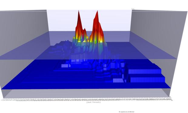
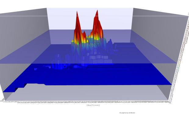
To turn my indicator into a trading system, I optimized buy and sell threshold (1-100) on SPY from 1/1/2000 – 12/29/2012. I optimized a long-only version of the system. Here is a picture of the 3D optimization with CAGR on the z-axis.

Buy Threshold

Sell Threshold

There is a small hilly region near the middle. I chose 40 as my buy threshold and 55 as my sell threshold since they are round numbers within the hilly region.

One thing peculiar that I noticed, but can’t seem to explain is that there are two of every set of system statistics, and the only difference is 1) the parameters of buy/sell threshold are switched and 2) the number of trades:

After some pondering I noticed that it might be because some of the buying is negligible. For example, if we have a 40/60 threshold then we will buy if the RSI is at 30, regardless if the 40 or the 60 is the buy threshold. However, the problem that I came across is that if the RSI is at 30 today, but is at 50 tomorrow, then we will buy & hold for a 40/60 threshold (buy when RSI < 40 and sell when RSI > 60), but we will buy & sell for a 60/40 threshold ( buy when RSI < 60 and sell when RSI > 40). I can’t seem to figure out why there each set of system statistics has a twin.

Next, I optimized the short and cover threshold (1-100) on the same data, using a short-only version of the system. Here is a picture of the 3D optimization with CAGR on the z-axis.

Short Threshold

Cover Threshold

There is another small hilly region near the middle. I chose 55 as my short threshold and 40 as my cover threshold since they are round numbers within the hilly region.

The peculiarity of the long only side of the system does not seem to exist on the short side.

Here is the optimized equity curve with a system of the following rules:

• Buy RSI < 40
• Sell RSI > 55
• Cover RSI < 40
• Short RSI > 55

The equity curve looks similar to that of many mean-reversion trading systems.

To check for robustness, I tested this system on multiple ETFs from 1/1/2000 – 12/29/2012.

For further robustness, I tested this system using different lengths of RSI on SPY.

One of my concerns is the success of the system since 2010, since many systems seemed to have performed differently or even completely stopped working from around that period. Here is the performance of the system on multiple markets from 1/1/2010 – 12/29/2012

Equity Curve Feedback

A concept that I thought of while showering a while back was treating an equity curve of a trading system as a tradeable security. It is analogous to using tactical asset allocation, except on trading systems instead of a portfolio of assets. Unfortunately for me, this is not a new idea. I also found this idea while going through the archives of my favourite blog, David Varadi’s CSS Analytics, and at Howard Bandy’s Quantitative Trading Systems in a post titled Equity Curve Feedback. So far, I’ve been able to think of four ways to apply this idea to a trading system, based on two types of equity curve feedback that I call “soft” and “hard” equity curve feedback.

• Soft equity curve feedback allows new trades to be entered when a certain equity condition is met.
• Hard equity curve feedback allows new trades to be entered when a certain equity condition is met AND forces new trades to be undertaken on the second derivative level while mid-trade on the first derivative level.

For example, say you are using an equity curve feedback rule that states that you will only trade when the the equity curve of System XYZ > 15 Day SMA of the equity curve of System XYZ . Your first trade on System XYZ manages to push the equity curve of System XYZ above its 15 Day SMA mid-way through the trade:

• With soft equity curve feedback entry, you are now allowed to trade System XYZ, but you do not enter the trade mid-way
• With hard equity curve feedback entry, you are now only allowed to trade System XYZ, but you also immediately enter the mid-way trade

With these two variations, we can come up with four different kinds of equity curve feedback overlays:

• Soft entry; Soft exit
• Hard entry; Soft exit
• Soft entry; Hard exit
• Hard entry; Hard exit

There are also two (three, but I don’t count one of them) forms of soft exits, but they aren’t different enough for me to classify it as an entirely different form of equity curve feedback.

• True soft exits – You cannot exit the system until the equity curve feedback condition is met. I do not consider this as a legitimate approach to equity curve feedback, since you are basically barred from exiting your system unless you are lucky.
• False soft exits – You can exit the system regardless of whether or not the equity curve feedback condition is met. You are not forced to exit your position if the equity curve condition turns from true to false, and you are still allowed to exit your position if the equity curve condition is false.
• Shorting soft exits – You can exit the system, but only based off of the inverse of your original trading system. For example, say System XYZ from above has the following rules
  • Buy: X > 10
  • Sell: X <10
  • Short: Y > 10
  • Cover: Y <10
  • X and Y are random indicators

  with the same 15-Day crossover equity curve feedback rules as before. You’re using hard entries and you entered in the first trade, but somewhere along the way the equity curve dipped below its 15 Day SMA. Now instead of exiting when X < 10, you exit when Y < 10. This only work if System XYZ has both long and short components, and you allow the shorting of the trading system itself.

From my experience (I’ve only played with it through back-testing, not live money. I’ve also only used simple SMA crossover trading strategies), equity curve feedback doesn’t really improve/detract from total CAGR (sometimes it improves/detracts but usually it maintains CAGR that is roughly similar), but it improves MDD and volatility.

QIM’s Jaffray Woodriff

Multiple quotes that I found useful:

I discovered that it was much better to use multiple models than a single best model.

Probably why he uses ensemble methods.

I started out using market-specific models. I ended up realizing that these models were far more vulnerable to breaking down in actual trading because they were more prone to being overfitted to the past data. In 1993, I started to figure out that the more data I used to train the models, the better the performance. I found that using the same models across multiple markets provided a far more robust approach. So the big change that occurred during this period was moving from separate models for each market to common models applied across all markets. The second change that occurred was increased diversification. I started out trading only two markets and then for some time traded only three markets. But as assets under management increased, and I realized it was best to use the same models across all markets, I added substantially more markets to the portfolio. The transition to greater diversification also helped improve performance. By 1994, I was trading about 20 markets, and I was no longer using market-specific models. Those changes made a big difference.

Diversifying across multiple markets is a commonly used tactic to prevent over-fitting, however I don’t particularly believe that a successful model is required to perform well on all markets, only markets that are similar (such as S&P500 & Nasdaq ETFs). Models that perform well in market A, but not int market B is not necessarily overfit, it only means that the particular model captures idiosyncratic behavior that is only observable in market A. I do agree that a model that successful across multiple markets will be more robust than one that is only successful in a handful of markets.

There are books about the predictive modeling process that specifically caution against “burning the data”—that is, you have to greatly limit the number of combinations you ever try. And I found that advice markedly stupid because I knew I could find a way to try any number of combinations and not overfit the data. You get new out-of-sample data every day. If you are rigorous about acknowledging what that new data is telling you, you can really get somewhere. It may take a while. If you are trading the system, and it is not performing in line with expectations over some reasonable time frame, look for overfit and hindsight errors. If you are expecting a Sharpe ratio above 1, and you are getting a Sharpe ratio under 0.3, it means that you have made one or more important hindsight errors, or badly misjudged trading costs. I was using the data up to a year before the current date as the training data set, the final year data as the validation data set, and the ongoing real-time data as the test. Effectively, the track record became the test data set.

Walk-forward testing before testing the system live with real money would be safer.

The first thing you need to do is to get some idea of how much of the apparent edge is completely spurious. Let’s say instead of training with the target variable, which is the price change over the subsequent 24 hours, I generate random numbers that have the same distribution characteristics. I know that any models that I find that score well training on this data are 100 percent curve-fitted because they are based on intentionally bogus data. The performance of the best model on the fictitious data provides a baseline. Then, you need to come up with models that do much better than this baseline when you are training on the real data. It is only the performance difference between the models using real data and the baseline that is indicative of expected performance, not the full performance of the models in training.

This, and monte-carlo simulations are good additional tests to prevent curve-fitting.

You can look for patterns where, on average, all the models out-of-sample continue to do well. You know you are doing well if the average for the out-of-sample models is a significant percentage of the in-sample score. Generally speaking, you are really getting somewhere if the out-of-sample results are more than 50 percent of the in-sample.

Cross-validate to protect against curve-fitting.

Sometimes we give a little more weight to more recent data, but it is amazing how valuable older data still is. The stationarity of the patterns we have uncovered is amazing to me, as I would have expected predictive patterns in markets to change more over the longer term.

I think there are idiosyncratic movements that are only existent in more recent data, but he uses older data to prevent (once again) prevent-curve fitting.

The core of the risk management is evaluating the risk of each market based on an exponentially weighted moving average of the daily dollar range per contract.

How he manages to keep so close to his volatility target.

– All quotes from Jaffray Woodriff in Hedge Fund Market Wizards

MR Swing System Development

Our system  design starts  with the  core principles  outlined  in the introduction: (1) we exploit different characteristics of markets by using a market‐regime‐switching method to take advantage of short‐term mean‐reversion in the bear regime, and deploy swing trading in the bull regime.  Next, we will employ (2)  non  symmetrical  trading  algorithms  for  entries,  exits  and  the  regime  specific  trading  algorithms. Every system component must be based on (3) volatility adaptive metrics so that it can handle changes in volatility over a long time span.  Finally, we recognize that no regime switching model will be able to  eliminate  all  false  signals  and  each  core  system  component  must  exhibit  (4)  robustness  to  regime whipsaws.

– from MR Swing