I came across the paper “Embedded Leverage” by Andrea Frazzini and Lasse Heje Pedersen. I didn’t have time to read it, but skimming over the abstract did spark some ideas from a previous paper I read. In the abstract, it states “we find that asset classes with embedded leverage offer low risk-adjusted returns and, in the cross-section, higher embedded leverage is associated with lower returns. A portfolio which is long low-embedded-leverage securities and short high-embedded-leverage securities earns large abnormal returns, with t-statistics of 8.6 for equity options, 6.3 for index options, and 2.5 for ETFs.” This made me think of a previous paper I read, titled “Alpha Generation and Risk Smoothing using Volatility of Volatility” by Tony Cooper. In that paper, he talks about “Volatility Drag”, which is the deterioration of performance due to volatility, which can be seen by the following formula:
(1-x)(1+x) = 1-x^2
In leveraged ETFs, this volatility drag effect is amplified.
Thinking about both of those papers made me hypothesize that a portfolio consisting of shorting 3x leveraged ETFs could perform extremely well from two factors:
- The high “embedded leverage”
- The increased volatility drag
To test this hypothesis out, I backtested 3 systems shorting pairs of 3x leveraged ETFs. The pairs were chosen so that there was 1 inverse ETF and 1 regular, and that they were created by the same company. I chose inverse/non-inverse pairs so that the majority of the movements would cancel each other out and create a smoother equity curve, and I chose ETFs from the same company so that the pairs would have similar (but inverse) indexing methodologies. The positions were rebalanced daily using adjusted close prices from Yahoo! Finance. Commission and slippage were not accounted for. The ETF pairs are:
- UPRO/SPXU
- FAZ/FAS
- GASL/GASX
- RUSS/RUSL
- TECL/TECS
There was no reason these particular ETFs were chosen. I just went to ETFdb.com and screened for 3x leveraged equity ETFs and ranked the ETFs by AUM. Then I chose a couple pairs.


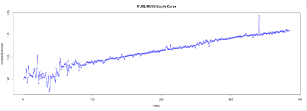


While viewing these charts keep in mind that the testing period for some ETFs were longer than others, which will affect cumulative return.The returns for most of them are mediocre at best, but the equity curve is relatively stable. What worries me is the pair TECL/TECS. While such a drop has only occurred to 1/5 of these pairs, this kind of black swan event could ruin the strategy and is enough to warrant not implementing the strategy.
Next I will try to find evidence that the returns are derived increased volatility drag through by plotting the rolling 10-day return of the strategy with the rolling 10-day historical volatility of the strategy.

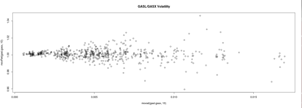
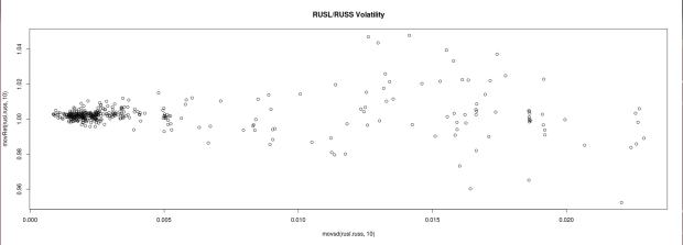


From a cursory glance, volatility doesn’t seem to be a huge predictor of returns in any of the pairs except for FAS/FAZ.
Conclusion:
This strategy doesn’t generate enough alpha to warrant trading IMO. Even though it has a stable equity curve (depending on the securities traded) black swan events such as the one that occurred in TECS/TECL can devastate the already small profits. This combined with the fact that the system trades extremely frequently (once per day) and thus has relatively large commissions should counter-act any benefits the strategy has. Other than researching if the volatility of 1 of the ETFs is a predictor of future returns, I’m not sure where else to continue researching/developing this strategy. If anyone has any thoughts/ideas please feel free to share 🙂
Side Note: This is the first time I’m using R. Everything should be calculated correctly, but I’m posting the code for this strategy so someone can point out an error in case I calculated something incorrectly.
# Function
getInvRet <- function(x) #Gets Inverse Daily Return
{
    raw.close <- read.csv(x) # read from CSV
    close <- raw.close[,7] # get Adjusted Close
    close <- rev(close) # flip the data
    ret <- close[-1]/close[-1*length(close)] # convert to daily ret
    inverse.ret <- -1*(ret-1) + 1 # inverse it for shorting
    inverse.ret
}
getPairRet <- function(retA, retB) #Calculates Shorting Rebalance Return
{
    equity <- retA * .5 + retB * .5
    equity <- c(1,equity)
    equity
}
movsd <- function(equity,lag) #Rolling Standard Deviation
{
    movingsd <- vector(mode="numeric",length(equity)-lag+1)
    for(i in lag:length(equity)) {movingsd[i-lag+1] <-sd(equity[(i-lag+1):i])}
    movingsd
}
movRet <- function(equity,lag) #Rolling Returns
{
    #for(i in 1:lag){}
    #for(i in length(equity)-lag+1:length(equity){}
    equity <- cumprod(equity)
    movingRet <- vector(mode="numeric",length(equity)-lag+1)
    for(i in lag:length(equity)) {movingRet[i-lag+1] <-equity[i]/equity[(i-lag+1)]} # this should be vectorized
    movingRet

}
#Get Inverse Returns
ret.fas <- getInvRet("fas.csv")
ret.faz <- getInvRet("faz.csv")
ret.gasl <- getInvRet("gasl.csv")
ret.gasx <- getInvRet("gasx.csv")
ret.rusl <- getInvRet("rusl.csv")
ret.russ <- getInvRet("russ.csv")
ret.spxu <- getInvRet("spxu.csv")
ret.upro <- getInvRet("upro.csv")
ret.tecl <- getInvRet("tecl.csv")
ret.tecs <- getInvRet("tecs.csv")

#Get Short Leverage Equity Curve
fas.faz <- getPairRet(ret.fas,ret.faz)
gasl.gasx <- getPairRet(ret.gasl,ret.gasx)
rusl.russ <- getPairRet(ret.rusl,ret.russ)
spxu.upro <- getPairRet(ret.spxu,ret.upro)
tecl.tecs <- getPairRet(ret.tecl,ret.tecs)