Mean-Reversion Volatility Filters Part Two: Since 2011

On my previous post, Mean-Reversion Volatility Filters, I used a dynamic volatility filter to filter out trades within  a short-term mean reversion system. I came to the conclusion that low vol was conducive for short term mean reversion performance. However, it’s commonly discussed how the market has shifted dynamics some time after the 2007-2008 financial crisis. In this post I revisit the tests ran in my previous post, testing from 1/1/2011 – 4/28/2013 rather than 1/1/1995 – 4/28/2013. The charts displayed below are 10-trade moving average of % profit from 1/1/1995-4/28/2013.

Results

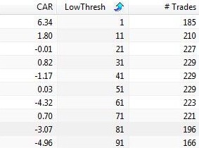
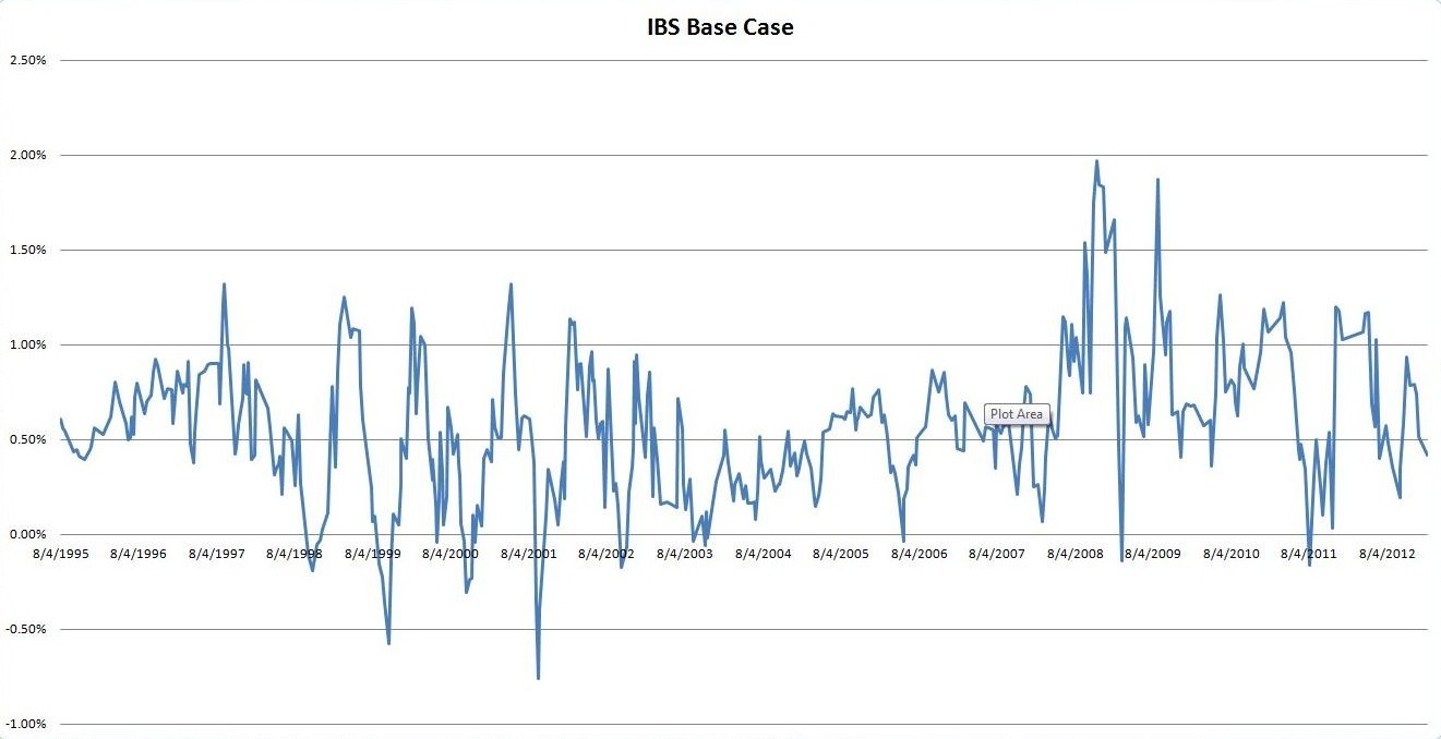
IBS

Rules (Base-Case):

• Buy if 3-Day IBS < 40
• Sell if 3-Day IBS > 40
• Avg. Trade: 0.53%

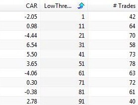
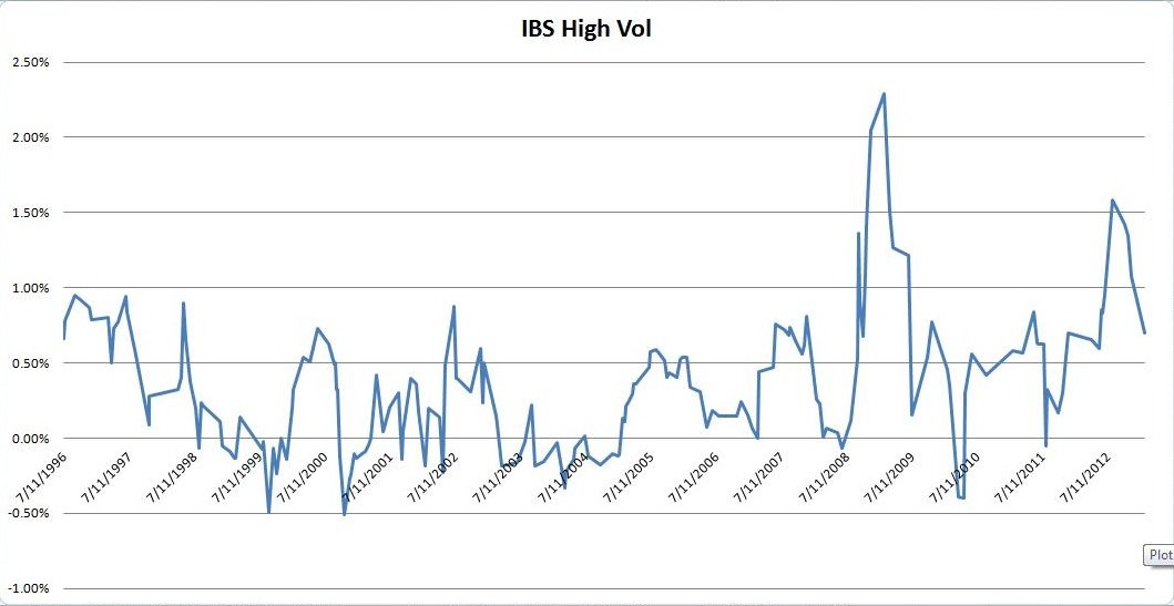
Rules (High Vol):

• Buy if 3-Day IBS < 40 AND HV(5) > HV(20)
• Sell if 3-Day IBS > 40
• Avg. Trade: 0.68%

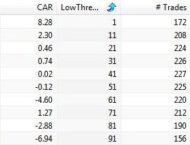
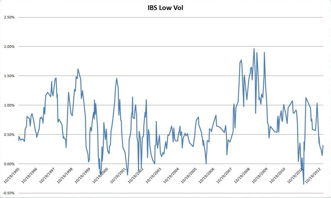
Rules (Low Vol):

• Buy if 3-Day IBS < 40 and HV(5) < HV(20)
• Sell if 3-Day IBS > 40
• Avg. Trade: 0.38%

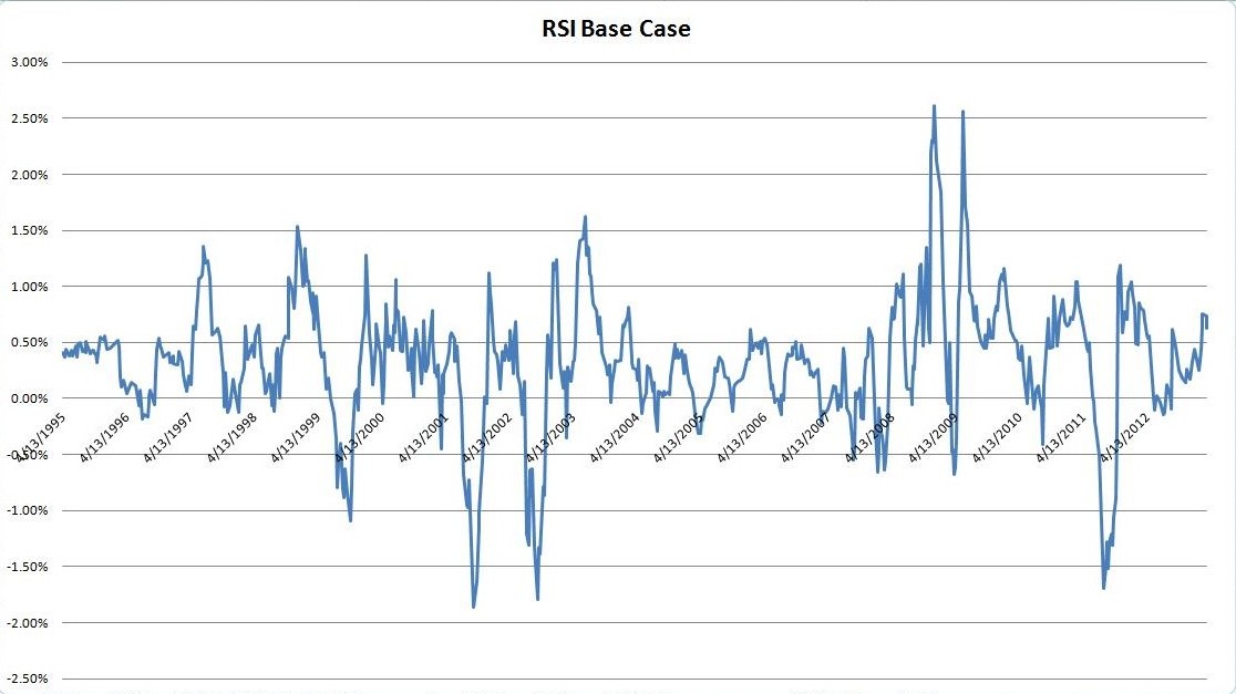
RSI

Rules (Base-Case):

• Buy if 2-Day RSI< 50
• Sell if 2-Day RSI > 50
• Avg. Trade: 0.21%

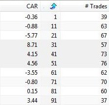
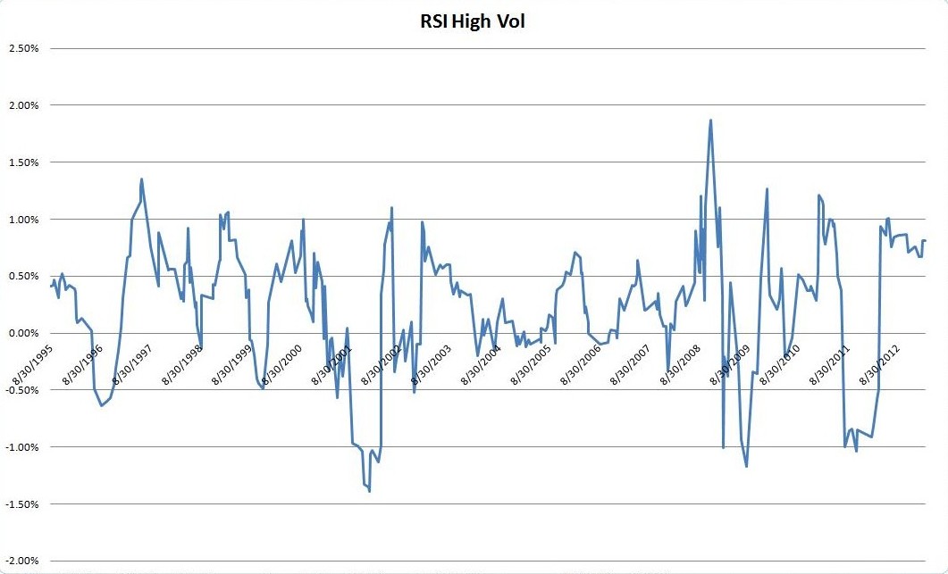
Rules(High Vol):

• Buy if  2-Day RSI< 50 and HV(5) > HV(20)
• Sell if 2-Day RSI > 50
• Avg. Trade: 0.40%

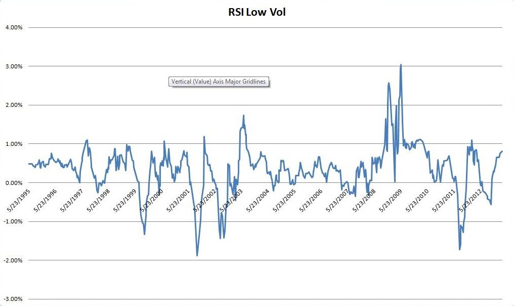
Rules(Low Vol):

• Buy if  2-Day RSI< 50 and HV(5) < HV(20)
• Sell if 2-Day RSI > 50
• Avg. Trade: 0.10%

Conclusion

Without looking at the charts, it may seem like post 2011, this volatility filter, like many strategies, has completely changed. However after looking at the charts of a rolling 10-trade moving average of % profit. the results become more inconclusive. It seems much more likely that the short term test results are due to unrepresentative and small sample size, rather than a change in volatility filter performance.

 

Mean-Reversion Volatility Filters

Due to the result’s of this MarketSci post, which imply that short-term mean reversion performs better during low volatility versus high volatility, I decided to revisit volatility filters. In Mean-Reversion within Regimes, I previously concluded that high volatility, not low volatility was more conducive to mean-reversion strategies. To test for low volatility/high volatility I decided to use a different filter. Last time I used a static test (60-Day Historical Volatility > 0.01 = High Volatility, <0.01 = Low Volatility). This time I will use a more dynamic filter, which compares short-term volatility to mid-term volatility.

Results

• Testing on SPY from 1/1/1995- 4/28/2013

IBS

Rules (Base-Case):

• Buy if 3-Day IBS < 40
• Sell if 3-Day IBS > 40
• Avg. Trade: 0.56%

Rules (High Vol):

• Buy if 3-Day IBS < 40 AND HV(5) > HV(20) 
• Sell if 3-Day IBS > 40
• Avg. Trade: 0.39%

Rules (Low Vol):

• Buy if 3-Day IBS < 40 and HV(5) < HV(20)
• Sell if 3-Day IBS > 40
• Avg. Trade: 0.68%

RSI

Rules (Base-Case):

• Buy if 2-Day RSI< 50
• Sell if 2-Day RSI > 50
• Avg. Trade: 0.32%

Rules(High Vol):

• Buy if  2-Day RSI< 50 and HV(5) < HV(20)
• Sell if 2-Day RSI > 50
• Avg. Trade: 0.27%

Rules(Low Vol);

• Buy if  2-Day RSI< 50 and HV(5) < HV(20)
• Sell if 2-Day RSI > 50
• Avg. Trade: 0.37%

Conclusion

It seems from this, in combination with my previous conclusion from Mean-Reversion within Regimes, that the specific filter used for volatility has a large influence on profitability. One thing I realized is that there may be different exposures for low vol vs high vol (meaning that a high volatility filter may allow for more trades, resulting in a higher CAGR) which could result in the discrepancy in results (that is why I used Avg. Trade rather than CAGR this time), but even after re-running the different tests under the same conditions, high vol had a higher Avg. Trade vs low vol.

A New Approach to Trading

Recently I changed the way I approach trading system development. Reading A Different Approach to Money Management is what gave me the original idea to alter my approach to trading, but my research is what pushed me over the edge.

Old Way

I approached trading system development with the goal of trying to develop a system with maximum exposure. I didn’t think of running two systems at the same time on the same pool of money (without splitting up the money) if the systems had little/no conflicting signals. Since most of the systems I tested on SPY either had either:

• high exposure but low returns
• high returns (after factoring for exposure) but low exposure

I was left with trying to develop a new system, or trying to trade the system over a large group of stocks (I used the Nasdaq-100 as my stock universe). While I was able to ramp up my exposure to around 70% with any system I tested, I often had to trade 5 or more stocks just to have a reasonable draw-down, which meant that commissions ate a large percent of my trading profits, considering my systems were short term in nature and I have limited capital.

Pros:

• Only one system to manage
• I don’t have to check for as many signals

Cons:

• Not diversified – higher risk
• High commissions due to being forced to trade many stocks to increase exposure
• Can be curve fit easily since I try to develop one super-system
• Higher model risk – there is only one model, which can fail at any given time

New Way

Now, I try to develop multiple systems that have high average profit% per trade with little/no regard for exposure. Even if the system trades only once every two or three months, I can combine many of these systems to trade at a frequency I would be trading at with my old way, but still maintain a highly profitable trading system with lower risk (assuming the systems do not have perfect correlation). While it’s too soon to draw any conclusions from live performance, the historical backtest shows dramatically improved results.

Pros

• Higher returns
• Lower risk
• Lower commissions since I only have to trade one stock (I trade SPY)
• Less risk of curve-fit – I will not be forced to include multiple filters to decrease risk/increase returns
• Lower model risk – chances of multiple models of failing is lower than one model failing

Cons

• Much more of a headache to manage when entering in trades EOD

Mean Reversion Trading in Moderation

Simple mean-reversion trading strategies in US equities have performed poorly since 2010/2011. Mean reversion is not dead, it never will be, but it may expressed differently than previously. Mean reversion prior to 2010, existed mainly in the form of extremes. The more extreme a pullback, the higher chance for a huge reversal. To test this, I ran 10 different frictionless  tests on SPY (from Yahoo! Finance) from 1/1/2000 – 1/1/2010.

Rules:

• Buy if the 250-day DV2 is greater than a threshold AND if it is less than the threshold + 10 (this means I will only buy if the DV2 is within a certain 10 point range).
• Sell the next day.
•  It is worth noting here that I have an option on in AmiBroker that prevents me from entering buy orders the same day that I enter sell orders, which will lower the overall exposure of these systems.

Here are the results:

We can clearly see that the returns are largely derived from the 1-11 bucket, meaning that extreme mean reversion was the source of returns. In the past 3 years, mean reversion exists in more moderate forms. Extreme pullbacks no longer indicate large reversals, but moderate pullbacks are more indicative of future gains. To test this, I ran the same test from 1/1/2010 – 1/1/2013:

The returns for the past three years are from the 31-41, 41-51, and 51-61 bucket. The 1-11 bucket went from a 6% CAGR to a -2% CAGR.

Here are the rules for another test I ran. This should be the result of the above rules if I allowed entries to be entered the same day as exits.

Rules:

• Buy if the 250-day DV2 is greater than a threshold AND if it is less than the threshold + 10 (this means I will only buy if the DV2 is within a certain 10 point range).
• Sell if the 250-day DV2 is less than a threshold OR if it is more than the threshold + 10

Results for 1/1/2000 – 1/1/2010:

Results for the same test for 1/1/2010 – 1/1/2013:

This is only a preliminary test over SPY, but it does lead to avenues for further research.